論文タイトルのテキスト解析 (RMeCab)
昨日のコードを転用して、論文タイトルでテキスト解析
- タイトル中での出現頻度が高い語句は?
- タイトル中での出現頻度が増えている語句は?
- 各誌で掲載される論文の傾向は?
library(tidyverse) # ggplotとかdplyrとか
library(rvest) # webスクレイピング用
library(XML) # rvestで必要なので
library(magrittr)
library(stringr) # 文字列操作用
library(data.table)
library(RMeCab)
library(wordcloud2)
library(knitr)
library(broom)
library(foreach)
library(pforeach)

# 雑誌リスト
NP <- "1469-8137" #New Phytologist
PCE <- "1365-3040"  # Plant, Cell & Environment
PJ <- "1365-313X" # The Plant Journal
PP <- "1399-3054" # Physiologia Plantarum
PB <- "1438-8677" # Plant Biology

# 作業用フォルダを作って移動
setwd("/Users/keach/Dropbox/KeachMurakami.github.io/_source/")
dir.create("2016-12-26")
setwd("2016-12-26")
解析
- 対象は前回同様、Wileyの植物系の5誌
- 各誌100号分のタイトルを取得
- 雑誌によって発行頻度が違うので、解析期間も違う
- 古いものだと1998年あたりのデータから解析
- 途中で雑誌名が代わっているものは、変更前を省略
- 各誌100号分のタイトルを取得
- 日本語形態素解析器MeCab1をR経由 (RMeCab2経由) で動かして、テキストマイニング
# 並列計算で5誌の100号をスクレイプ
title_list <-
  pforeach(i = c(NP, PCE, PJ, PP, PB), .combine = bind_rows)({
    extract_ISSN(ISSN = NP, number_parse = 100)
  })

title_df <-
  title_list %>%
  tidyr::extract(col = title, into = c("title", "start", "end"), regex = "(.+)\\(pages(.+[0-9]+)–([0-9]+)") %>% # remove pages
  tidyr::extract(col = issue_volume, into = c("vol", "issue"), regex = "([0-9]+).+([0-9]+)") %>% # separate volume and issue
  tidyr::extract(col = date, into = c("month", "year"), regex = "([a-zA-Z]+).([0-9]+)") # separate month and year

# csvで保存
title_df %>%
  write_csv(path = "./titles_scrape.csv")
}
pforeach3による並列計算が簡単で素晴らしい- scrape処理の並列化で実行時間がざっくり1/2
# 非並列計算
system.time(
  lapply(
    c(NP, PCE, PJ, PP, PB), function(i){
      extract_ISSN(ISSN = i, number_parse = 5)
      })
  )

 #   user  system elapsed
 # 10.365  38.943  53.938


# 4コア並列計算
system.time(
  pforeach::pforeach(i = c(NP, PCE, PJ, PP, PB), .combine = bind_rows)({
    extract_ISSN(ISSN = i, number_parse = 5)
    })
  )

  #  user  system elapsed
  # 5.508  15.315  24.520
テキストマイニング
- 品詞で解析とか、ステム (photosynthesis と photosynthetic のような関係性) の解析とか、気になるけど放置
- 英語タイトルの解析だからそもそもMeCab (日本語用) を使うのが愚かだった
- MeCabがファイルからしか解析できないので、一時ファイル出力、という感じ
titles <-
  fread("./titles_scrape.csv") %>%
  as_data_frame %>%
  filter(!(journal %in% c("Acta Botanica Neerlandica", "Botanica Acta"))) %>% # 雑誌名の変更前のものを除く
  mutate(title = tolower(title)) # 全て小文字に

# 品詞で解析したかったけど...
RemoveList <-
  c("of", "in", "on", "to", "for", "by", "with", "from",
    "at", "among", "but", "or", "into", "under", "via", "during",
    "and", "is", "are", "as", "between", "that", "its", "their",
    "the", "a", "an")

titles_grouped <-
  titles %>%
  group_by(journal, year) %>%
  do(
    .$title %>%
    paste(collapse = " ") %>%
    data_frame(title = .)
  )

titles_freqs <-
  foreach(i = 1:dim(titles_grouped)[1], .combine = bind_rows) %do%
  {
    df_slice <-
      titles_grouped[i, ]

    # MeCabがファイルからしか解析できないので、一時ファイルを吐く
    df_slice %$%
      title %>%
      write.table(file = "temp.txt", row.names = F, col.names = F)

    # MeCabる
    journal <- df_slice$journal
    year <- df_slice$year

    # 整える
    result_mecab <-
      "temp.txt" %>%
      RMeCabFreq %>%
      filter(Info1 != "記号", Info2 == "一般", !(Term %in% RemoveList)) %>%
      mutate(journal = journal, year = year) %>%
      select(term = Term, freq = Freq, journal, year) %>%
      return
  }
## file = temp.txt
## length = 846
## file = temp.txt
## length = 2084
## file = temp.txt
## length = 2066
## file = temp.txt
## length = 2221
## file = temp.txt
## length = 2243
## file = temp.txt
## length = 2339
## file = temp.txt
## length = 2520
## file = temp.txt
## length = 2618
## file = temp.txt
## length = 2719
## file = temp.txt
## length = 2766
## file = temp.txt
## length = 727
## file = temp.txt
## length = 798
## file = temp.txt
## length = 1047
## file = temp.txt
## length = 1212
## file = temp.txt
## length = 1227
## file = temp.txt
## length = 1163
## file = temp.txt
## length = 955
## file = temp.txt
## length = 918
## file = temp.txt
## length = 834
## file = temp.txt
## length = 946
## file = temp.txt
## length = 1091
## file = temp.txt
## length = 1165
## file = temp.txt
## length = 1001
## file = temp.txt
## length = 919
## file = temp.txt
## length = 147
## file = temp.txt
## length = 744
## file = temp.txt
## length = 730
## file = temp.txt
## length = 642
## file = temp.txt
## length = 760
## file = temp.txt
## length = 671
## file = temp.txt
## length = 689
## file = temp.txt
## length = 707
## file = temp.txt
## length = 730
## file = temp.txt
## length = 722
## file = temp.txt
## length = 796
## file = temp.txt
## length = 970
## file = temp.txt
## length = 923
## file = temp.txt
## length = 1067
## file = temp.txt
## length = 1030
## file = temp.txt
## length = 1062
## file = temp.txt
## length = 1031
## file = temp.txt
## length = 1267
## file = temp.txt
## length = 1058
## file = temp.txt
## length = 137
## file = temp.txt
## length = 592
## file = temp.txt
## length = 1008
## file = temp.txt
## length = 1281
## file = temp.txt
## length = 930
## file = temp.txt
## length = 1092
## file = temp.txt
## length = 1061
## file = temp.txt
## length = 1199
## file = temp.txt
## length = 1169
## file = temp.txt
## length = 1063
## file = temp.txt
## length = 1233
## file = temp.txt
## length = 1406
## file = temp.txt
## length = 1494
## file = temp.txt
## length = 1471
## file = temp.txt
## length = 174
## file = temp.txt
## length = 1002
## file = temp.txt
## length = 1948
## file = temp.txt
## length = 1896
## file = temp.txt
## length = 1971
## file = temp.txt
## length = 2005
## file = temp.txt
## length = 1958
## file = temp.txt
## length = 1403
# 解析結果をcsvで保存
titles_freqs %>%
  write_csv(path = "titles_analyzed.csv")
データ解析・可視化
全体
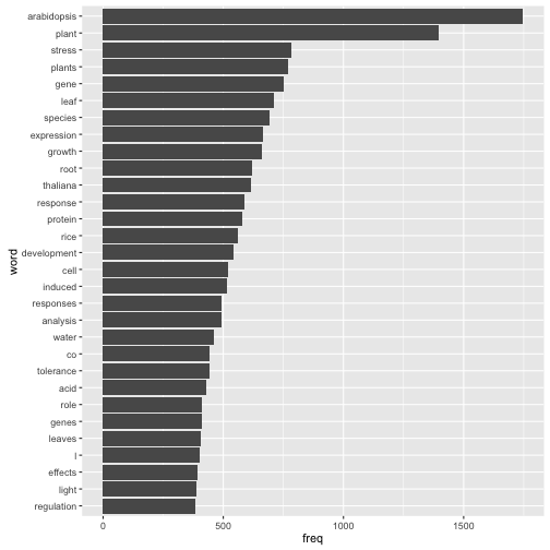
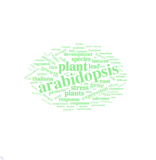
- 解析期間を通しての出現回数のトップ30までの単語を表示、全単語をWordCloud化
- Arabidopsis thaliana (シロイヌナズナ) がつよい
- その他の固有名詞だと、riceくらい
- coはたぶんCO2
- lってなんだ、と思ったら、種名をつけたLinnéのL
- WordCloudはおしゃれだけど得られるものは少ない
- Arabidopsis thaliana (シロイヌナズナ) がつよい
freqs_all <-
  titles_freqs %>%
  group_by(term) %>%
  summarise(freq = sum(freq))

# 出現総数TOP30
freqs_all %>%
  arrange(desc(freq)) %>%
  head(30) %>%
  ggplot(aes(x = reorder(term, freq), y = freq)) +
  geom_bar(stat = "identity") +
  coord_flip() +
  labs(x = "word")
# ワードクラウド
freqs_all %>%
  arrange(desc(freq)) %>%
  wordcloud2(size = .3, color = "lightgreen")
計時推移
- 頻出30単語を抽出して、計時推移をプロット
- 総単語数 (上図) が増えているため、割合にして確認 (下図)
major_terms <-
  freqs_all %>%
  arrange(desc(freq)) %>%
  head(30) %$%
  term

# 年ごとの出現word総数
terms_per_year <-
  titles_freqs %>%
  filter(term %in% major_terms) %>%
  group_by(year) %>%
  summarise(total = sum(freq))

time_dat <-
  titles_freqs %>%
  filter(term %in% major_terms) %>%
  group_by(year, term) %>%
  summarise(freq = sum(freq)) %>%
  left_join(., terms_per_year, by = "year") %>%
  filter(year != "2017") %>%  # 2017年はデータがまだ少ないので除外
  mutate(freq_percent = freq / total) %>%
  gather(category, freq, -year, -term) %>%
  filter(category != "total")

# 経年推移
time_dat %>%
  ggplot(aes(x = year, y = freq, col = term)) +
  geom_line() +
  geom_point() +
  facet_grid(category ~ ., scale = "free")
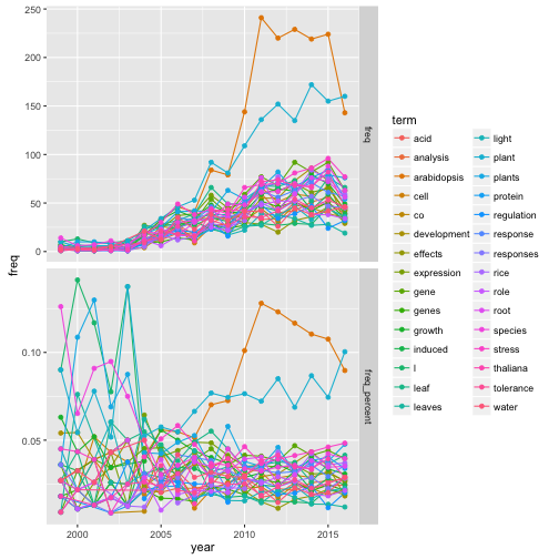
- Arabidopsisの時代は過ぎた?
- 転換期 (2011年) 以降の推移を線形回帰 (雑) すると、genes・expressionも同時期に低下傾向
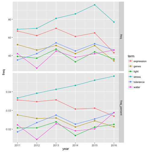
- 時代はstress応答 (stress・water・tolerance)
- 雑な解析ではあるが、感覚には即している
- この気運を状態空間モデルなんかで表現できると面白い
# 線形回帰でごり押し
time_dat %>%
  filter(year > 2010, category == "freq_percent") %>%
  rename(Term = term) %>%
  group_by(Term) %>%
  do(lm(data = ., formula = freq ~ year) %>% tidy) %>%
  filter(term == "year") %>%
  select(term = Term, increase = estimate, p = p.value) %>%
  mutate(signif = if_else(p < 0.05, "*", "")) %>%
  arrange(desc(increase)) %>%
  kable
| term | increase | p | signif |
|---|---|---|---|
| plant | 0.0036254 | 0.2317952 | |
| stress | 0.0023209 | 0.0000007 | * |
| species | 0.0015994 | 0.0664947 | |
| effects | 0.0015518 | 0.0673976 | |
| tolerance | 0.0014971 | 0.0803743 | |
| acid | 0.0013253 | 0.0868604 | |
| water | 0.0013107 | 0.2928148 | |
| plants | 0.0012870 | 0.4527388 | |
| l | 0.0012478 | 0.1174085 | |
| leaf | 0.0003580 | 0.8030076 | |
| root | 0.0003429 | 0.8327486 | |
| response | 0.0003360 | 0.6385665 | |
| rice | 0.0003153 | 0.8237002 | |
| responses | 0.0002245 | 0.7495239 | |
| gene | 0.0001728 | 0.8496393 | |
| induced | 0.0001078 | 0.9237296 | |
| light | 0.0000957 | 0.8911893 | |
| protein | 0.0000807 | 0.9239947 | |
| growth | -0.0000847 | 0.9332585 | |
| analysis | -0.0000983 | 0.9274333 | |
| co | -0.0001330 | 0.8662355 | |
| cell | -0.0009685 | 0.2177663 | |
| development | -0.0010298 | 0.6674606 | |
| leaves | -0.0011214 | 0.1942427 | |
| genes | -0.0011419 | 0.0486900 | * |
| regulation | -0.0013069 | 0.3054110 | |
| thaliana | -0.0015378 | 0.1778314 | |
| expression | -0.0016671 | 0.0132805 | * |
| role | -0.0017336 | 0.0901148 | |
| arabidopsis | -0.0069762 | 0.0019724 | * |
# いくつの単語の最近のトレンドに注目
time_dat %>%
  filter(term %in% c("genes", "expression", "tolerance", "water", "stress", "light", "temperature"),
         year > 2010) %>%
  ggplot(aes(x = year, y = freq, col = term)) +
  geom_line() +
  geom_point() +
  facet_grid(category ~ ., scale = "free")
雑誌ごとの色
- 各誌の頻出単語を30位まで
- New Phytologistは他と毛色が違う
- 菌類 (fungal・mycorrhizal) 系の話が多い
- いわれてみると、菌との相互関係だとかbiome系の論文は最近よくみかける気がする
- が、まったく読んでない
- たまには読んでみよう
- root・soil・evolution・forestとスケールがでかい
- 菌類 (fungal・mycorrhizal) 系の話が多い
- Physiologia PlantarumとPCEは環境応答系に注力している
- tolerance・drought・water・light・CO2
- 光合成関係だとやっぱりこのふたつ
- The Plant Journalは完全にMolecularな感じ
- 個人的にはあまり読んでも楽しくない (分子細胞生物学に弱い) ので敬遠しがち
- Plant Biologyは傾向がとりづらい
- 良く言えば間口が広い、悪く言えば軸がぶれている
- 花粉系…? (pollen, pollination)
- New Phytologistは他と毛色が違う
titles_freqs %>%
  group_by(journal, term) %>%
  summarise(freq = sum(freq)) %>%
  do(arrange(., desc(freq)) %>%
       head(30) %>%
       mutate(rank = 1:30)) %>%
  ungroup %>%
  transmute(journal, term = paste0(term, " (", freq, ")"), rank) %>%
  spread(journal, term) %>%
  kable
| rank | New Phytologist | Physiologia Plantarum | Plant Biology | Plant, Cell & Environment | The Plant Journal |
|---|---|---|---|---|---|
| 1 | plant (632) | stress (250) | l (201) | arabidopsis (338) | arabidopsis (725) |
| 2 | arabidopsis (395) | arabidopsis (181) | plant (201) | leaf (247) | protein (239) |
| 3 | species (271) | expression (177) | species (174) | stress (232) | gene (209) |
| 4 | plants (270) | plant (160) | plants (138) | plant (200) | plant (203) |
| 5 | root (238) | gene (142) | growth (109) | water (193) | thaliana (187) |
| 6 | leaf (210) | response (137) | arabidopsis (108) | growth (176) | development (182) |
| 7 | gene (203) | plants (133) | effects (106) | co (170) | rice (173) |
| 8 | carbon (177) | induced (131) | seed (95) | root (162) | cell (165) |
| 9 | evolution (174) | growth (116) | stress (95) | response (161) | expression (138) |
| 10 | mycorrhizal (172) | leaf (112) | gene (94) | tolerance (159) | genes (121) |
| 11 | growth (160) | tolerance (107) | expression (90) | c (152) | required (117) |
| 12 | thaliana (157) | leaves (104) | leaf (90) | responses (152) | analysis (105) |
| 13 | nitrogen (155) | drought (93) | two (84) | leaves (149) | genome (105) |
| 14 | co (154) | water (92) | different (82) | thaliana (147) | factor (104) |
| 15 | analysis (145) | acid (91) | analysis (74) | plants (138) | growth (100) |
| 16 | protein (145) | development (91) | development (72) | l (132) | transcription (99) |
| 17 | responses (141) | analysis (86) | genetic (71) | species (131) | involved (98) |
| 18 | soil (140) | rice (86) | cell (67) | photosynthesis (129) | biosynthesis (97) |
| 19 | cell (139) | effects (85) | response (67) | light (126) | response (95) |
| 20 | development (138) | responses (83) | pollen (66) | rice (126) | stress (95) |
| 21 | expression (137) | root (82) | pollination (66) | induced (125) | plants (90) |
| 22 | induced (137) | species (82) | variation (65) | expression (121) | role (90) |
| 23 | rice (132) | protein (81) | leaves (62) | acid (111) | root (90) |
| 24 | fungal (131) | cell (79) | water (62) | drought (110) | resistance (86) |
| 25 | response (130) | changes (79) | induced (61) | gene (102) | acid (84) |
| 26 | genetic (129) | characterization (78) | reproductive (61) | temperature (101) | auxin (83) |
| 27 | resistance (128) | high (78) | populations (58) | carbon (100) | proteins (82) |
| 28 | forest (125) | regulation (78) | responses (58) | signalling (98) | mediated (81) |
| 29 | roots (120) | genes (76) | germination (55) | regulation (95) | like (75) |
| 30 | tree (118) | temperature (75) | drought (54) | conductance (93) | signaling (75) |