ggplot2を再履修する
ggplot2を使いこなしたい
元ネタはr-wakalangのggplot2チャンネル
Rの初心者の域を脱していないが、自分にわかる (わかっているつもりになっている) 範囲には答えるようにしている
答える → プロが現れる → わかっていなかったことがわかる → ひとり赤面する → 勉強するのループが重要だ (たぶん)
今回もひとり赤面していたので、ggplot2を再履修する
お題
ggplot2縛りで、ヒストグラムの上に度数のテキストラベルを載せたい
どうせなので、こつこつためたマイデータ (研究室への出入などの記録およそ2年分) を可視化する
# データ読み込む
Timecard <-
  data.table::fread("~/Dropbox/R/my.data/TimeCard.csv")

# ざっとみる
Timecard %>% head
##        day week Arrive    Leave Event Alc
## 1: 8/30/14  Sat  13:30 24:20:00        NA
## 2: 8/31/14  Sun  14:30    22:15        NA
## 3:  9/1/14  Mon  09:59    19:52        NA
## 4:  9/2/14  Tue  09:56    21:10        NA
## 5:  9/3/14  Wed  09:58    20:58        NA
## 6:  9/4/14  Thu  08:15    22:10        NA
Timecard %>% str
## Classes 'data.table' and 'data.frame':	554 obs. of  6 variables:
##  $ day   : chr  "8/30/14" "8/31/14" "9/1/14" "9/2/14" ...
##  $ week  : chr  "Sat" "Sun" "Mon" "Tue" ...
##  $ Arrive: chr  "13:30" "14:30" "09:59" "09:56" ...
##  $ Leave : chr  "24:20:00" "22:15" "19:52" "21:10" ...
##  $ Event : chr  "" "" "" "" ...
##  $ Alc   : int  NA NA NA NA NA NA NA NA NA NA ...
##  - attr(*, ".internal.selfref")=<externalptr>
記録の付け方が良くないので、少しデータクレンジング
reshape2::meltに慣れてしまい、tidyr::gatherに未だに移行できないでいる
InOutLab <-
  Timecard %>%
  # {lubridate}あたりでどうにかなりそう、勉強する
  transmute(arrive = as.numeric(str_sub(Arrive, 1, 2)) + as.numeric(str_sub(Arrive, 4, 5)) / 60,
            leave = as.numeric(str_sub(Leave, 1, 2)) + as.numeric(str_sub(Leave, 4, 5)) / 60) %>%
  melt(id.vars = NULL)

InOutLab %>% str
## Classes 'data.table' and 'data.frame':	1108 obs. of  2 variables:
##  $ variable: Factor w/ 2 levels "arrive","leave": 1 1 1 1 1 1 1 1 1 1 ...
##  $ value   : num  13.5 14.5 9.98 9.93 9.97 ...
##  - attr(*, ".internal.selfref")=<externalptr>
可視化
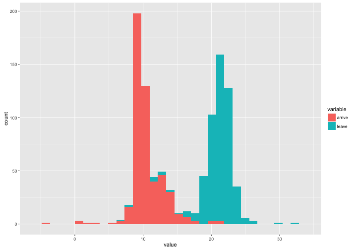
素直に表示
平日は9:00–10:00に研究室入りし、21:00–22:00に研究室を出ることが多い
InOutLab %>%
  ggplot(aes(x = value, fill = variable, group = variable)) +
  geom_histogram()
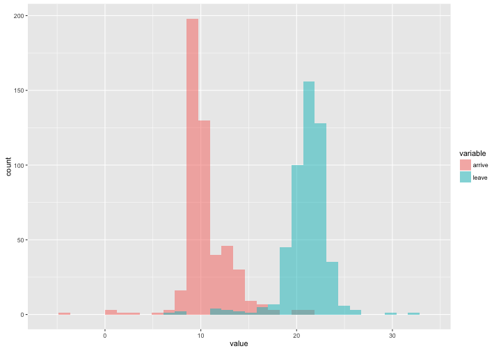
積み上げ表示の解除・透過率の指定
InOutLab %>%
  ggplot(aes(x = value, fill = variable, group = variable)) +
  geom_histogram(position = "identity", alpha = .5)
度数ラベルの追加
..count..で、ggplot2が内部で計算した結果として持っている度数を取ってくる
..XXX..はgenerated variables、あるいはcomputed variablesと呼ばれているらしい
stat = "bin"を指定しているのは、geom_text関数のデフォルトでは度数を計算してくれないから
こちらが詳しくて分かりやすかった
InOutLab %>%
  ggplot(aes(x = value, fill = variable, group = variable)) +
  geom_histogram(position = "identity", alpha = .5) +
  geom_text(aes(y = ..count.., label = ..count.., col = variable),
            stat = "bin")

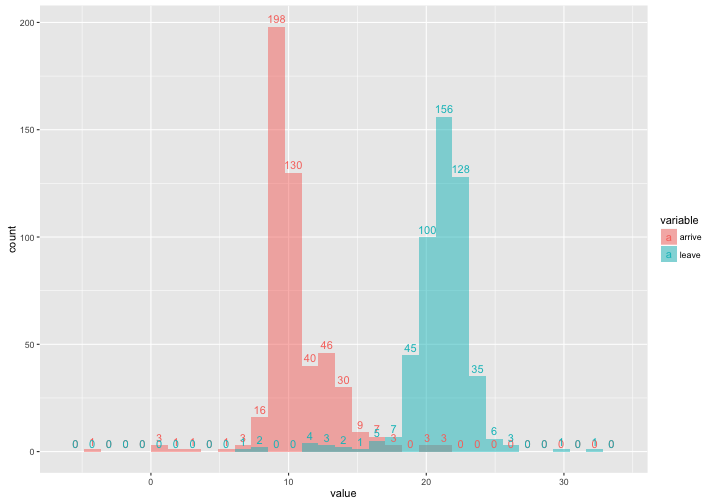
ラベル位置の調節
vjustで鉛直 (vertical) 方向の位置を調節 (adjust) する
InOutLab %>%
  ggplot(aes(x = value, fill = variable, group = variable)) +
  geom_histogram(position = "identity", alpha = .5) +
  geom_text(aes(y = ..count.., label = ..count.., col = variable),
            stat = "bin", vjust = -.5)

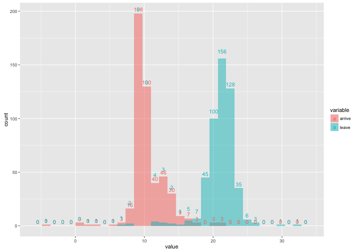
度数0を非表示
度数0の表示が邪魔なので非表示にする
ifelse関数を使って、..count.. > 0 なら..count..を、それ以外なら空白を返す
InOutLab %>%
  ggplot(aes(x = value, fill = variable, group = variable)) +
  geom_histogram(position = "identity", alpha = .5) +
  geom_text(aes(y = ..count.., label = ifelse(..count.. > 0, ..count.., ""), col = variable),
            stat = "bin", vjust = -.5)
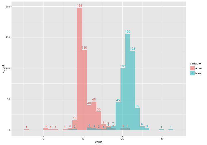
ひとまず完成
凝る
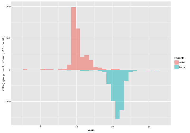
0で上下に分割
ifelse関数を使って、..group.. == 1(arriveが1、leaveが2) なら..count..を、それ以外なら-1 * ..count..を返す
InOutLab %>%
  ggplot(aes(x = value, fill = variable, group = variable)) +
  geom_histogram(aes(y = ifelse(..group.. == 1, ..count.., -1 * ..count..)),
                 position="identity", alpha = .5)
度数ラベルの追加
度数ラベルのy座標にもifelse関数を使って上下に分割
InOutLab %>%
  ggplot(aes(x = value, fill = variable, group = variable)) +
  geom_histogram(aes(y = ifelse(..group.. == 1, ..count.., -1 * ..count..)),
                 position="identity", alpha = .5) +
  geom_text(aes(y = ..count.. * ifelse(..group.. == 1, 1, -1), label = ifelse(..count.. != 0, ..count.., ""), col = variable),
            stat = "bin", vjust = -.5)

ラベル位置の調節
vjustを微調整
InOutLab %>%
  ggplot(aes(x = value, fill = variable, group = variable)) +
  geom_histogram(aes(y = ifelse(..group.. == 1, ..count.., -1 * ..count..)),
                 position="identity", alpha = .5) +
  geom_text(aes(y = ..count.. * ifelse(..group.. == 1, 1, -1), label = ifelse(..count.. != 0, ..count.., ""), col = variable, vjust = ifelse(..group.. == 1, -.5, 1.5)),
            stat = "bin")
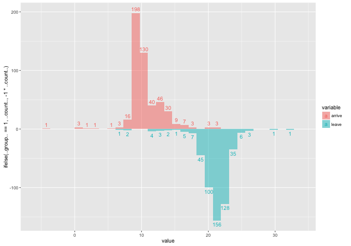
満足
3以上の変数がある場合には使えないが、2変数ならデータを捉えやすい
補足
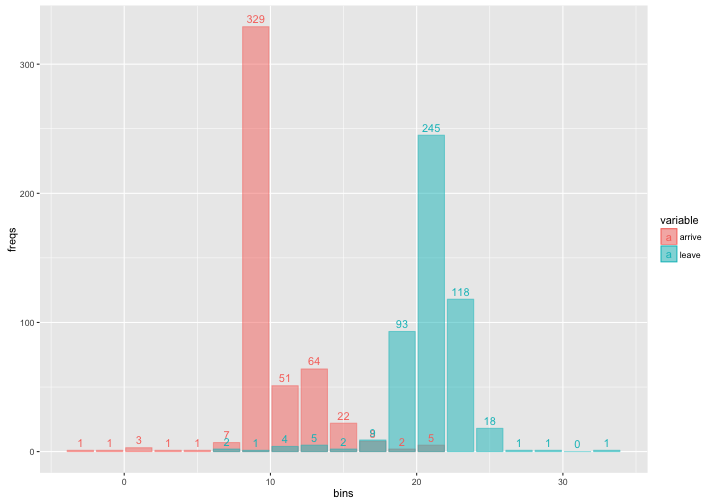
stat系は簡単な計算には便利だが速度は遅いため、大規模データの可視化では先にready plotな状態にしてからggplot2に渡した方がよいらしい
hist_ <-
  function(vec, algorithm = "Sturges"){
    x_bins <-
      vec %>%
        hist(., breaks = algorithm, plot = FALSE) %>%
        .[["breaks"]] %>%
        stats::filter(., c(1/2, 1/2)) %>%
        na.omit %>%
        as.vector

    x_counts <-
      vec %>%
        hist(., breaks = algorithm, plot = FALSE) %>%
        .[["counts"]]

    data.frame(bins = x_bins, freqs = x_counts) %>%
      return
  }

InOutLab %>%
  group_by(variable) %>% # groupごとにbinwidthが違うことがありえる仕様になっている
  do(.$value %>% hist_ %>% return) %>%
  ggplot(aes(x = bins, y = freqs, col = variable, fill = variable)) +
  geom_bar(stat = "identity", position = "identity", alpha = .5) +
  geom_text(aes(label = freqs), vjust = -.5)
NG集
generated variablesはaes()の中でしか呼べない
InOutLab %>%
  ggplot(aes(x = value, fill = variable, group = variable)) +
  geom_histogram(aes(y = ifelse(..group.. == 1, ..count.., -1 * ..count..)),
                 position="identity", alpha = .5) +
  geom_text(aes(y = ..count.. * ifelse(..group.. == 1, 1, -1), label = ifelse(..count.. != 0, ..count.., ""), col = variable),
            stat = "bin", vjust = ifelse(..group.. == 1, -.5, 1.5))

"Error in ifelse(..group.. == 1, -0.5, 1.5) : object '..group..' not found"
stat_bin(stat = “text”) とgeom_text(stat = “bin”) の違い
こちらのページで答えられている方法にしたがって、stat_bin()内でgeom = "text"を指定すると、うまくグループ化するとラベルが表示されない
InOutLab %>%
  ggplot(aes(x = value, fill = variable, group = variable)) +
  geom_histogram(position = "identity", alpha = .5) +
  stat_bin(aes(group = variable, y = ..count.., label = ..count.., col = variable), geom = "text", vjust = -.5)
stat_bin()では、geom_histogram()で指定したposition = "identity"を引き継いでおらず、ラベルの表示位置が積み上げ型の場合の表示位置になる
これを修正するためには、stat_bin()内でもposition = "identity"を指定する必要がある
冗長になるので、geom_text(stat = "bin")の方がよさそう?
わかった風になっていたがわかっていなかったので、キチンとstatとgeomの使い分けを勉強する必要がある
check!
InOutLab %>%
  ggplot(aes(x = value, fill = variable, group = variable)) +
  geom_histogram(position = "identity", alpha = .5) +
  stat_bin(aes(group = variable, y = ..count.., label = ..count.., col = variable), position = "identity", geom = "text", vjust = -.5)
# 参照用:
#  上で示したgeom_textを使った場合
#  geom_text()ではposition = "identity"を指定しなくてもOK
#
# InOutLab %>%
#   ggplot(aes(x = value, fill = variable, group = variable)) +
#   geom_histogram(position = "identity", alpha = .5) +
#   geom_text(aes(y = ..count.., label = ..count.., col = variable),
#             stat = "bin", vjust = -.5)
参考ページ
r-wakalangへようこそ (uriさん@Qiita)
ggplot2のgenerated variables(..変数名..)の使い方 (Technically, technophobic.@Hatena::Diary)
ggplot2で指定できるgenerated variableの一覧 (Technically, technophobic.@Hatena::Diary)
How to show count of each bin on histogram on the plot (Stack Overflow)
ggplot2再入門 (yutannihilationさん@SlideShare)
session_info()
##  setting  value
##  version  R version 3.2.3 (2015-12-10)
##  system   x86_64, darwin14.5.0
##  ui       X11
##  language (EN)
##  collate  en_US.UTF-8
##  tz       Asia/Tokyo
##  date     2016-03-05
##
##  package      * version    date       source
##  agricolae    * 1.2-3      2015-10-06 CRAN (R 3.1.3)
##  AlgDesign      1.1-7.3    2014-10-15 CRAN (R 3.1.2)
##  assertthat     0.1        2013-12-06 CRAN (R 3.1.0)
##  bitops       * 1.0-6      2013-08-17 CRAN (R 3.1.0)
##  boot           1.3-17     2015-06-29 CRAN (R 3.2.3)
##  chron          2.3-47     2015-06-24 CRAN (R 3.1.3)
##  cluster        2.0.3      2015-07-21 CRAN (R 3.2.3)
##  coda           0.18-1     2015-10-16 CRAN (R 3.1.3)
##  codetools      0.2-14     2015-07-15 CRAN (R 3.2.3)
##  colorspace     1.2-6      2015-03-11 CRAN (R 3.1.3)
##  combinat       0.0-8      2012-10-29 CRAN (R 3.1.0)
##  data.table   * 1.9.6      2015-09-19 CRAN (R 3.1.3)
##  DBI            0.3.1      2014-09-24 CRAN (R 3.1.1)
##  deldir         0.1-9      2015-03-09 CRAN (R 3.1.3)
##  devtools     * 1.9.1      2015-09-11 CRAN (R 3.2.0)
##  digest         0.6.8      2014-12-31 CRAN (R 3.1.2)
##  doParallel     1.0.10     2015-10-14 CRAN (R 3.1.3)
##  doRNG          1.6        2014-03-07 CRAN (R 3.1.2)
##  dplyr        * 0.4.3      2015-09-01 CRAN (R 3.1.3)
##  evaluate       0.8        2015-09-18 CRAN (R 3.1.3)
##  foreach      * 1.4.3      2015-10-13 CRAN (R 3.1.3)
##  formatR        1.2.1      2015-09-18 CRAN (R 3.1.3)
##  ggplot2      * 2.0.0      2015-12-18 CRAN (R 3.2.3)
##  gridExtra    * 2.0.0      2015-07-14 CRAN (R 3.1.3)
##  gtable       * 0.1.2      2012-12-05 CRAN (R 3.1.0)
##  httr           1.0.0      2015-06-25 CRAN (R 3.1.3)
##  iterators      1.0.8      2015-10-13 CRAN (R 3.1.3)
##  jsonlite       0.9.19     2015-11-28 CRAN (R 3.1.3)
##  klaR           0.6-12     2014-08-06 CRAN (R 3.1.1)
##  knitr        * 1.11       2015-08-14 CRAN (R 3.2.3)
##  labeling       0.3        2014-08-23 CRAN (R 3.1.1)
##  lattice        0.20-33    2015-07-14 CRAN (R 3.2.3)
##  lazyeval       0.1.10     2015-01-02 CRAN (R 3.1.2)
##  LearnBayes     2.15       2014-05-29 CRAN (R 3.1.0)
##  lubridate    * 1.5.0      2015-12-03 CRAN (R 3.2.3)
##  magrittr     * 1.5        2014-11-22 CRAN (R 3.1.2)
##  MASS         * 7.3-45     2015-11-10 CRAN (R 3.2.3)
##  Matrix         1.2-3      2015-11-28 CRAN (R 3.2.3)
##  memoise        0.2.1      2014-04-22 CRAN (R 3.1.0)
##  munsell        0.4.2      2013-07-11 CRAN (R 3.1.0)
##  nlme           3.1-122    2015-08-19 CRAN (R 3.2.3)
##  pforeach     * 1.3        2015-12-21 Github (hoxo-m/pforeach@2c44f3b)
##  pkgmaker       0.22       2014-05-14 CRAN (R 3.1.3)
##  plyr         * 1.8.3      2015-06-12 CRAN (R 3.1.3)
##  R6             2.1.1      2015-08-19 CRAN (R 3.1.3)
##  RColorBrewer * 1.1-2      2014-12-07 CRAN (R 3.1.2)
##  Rcpp           0.12.2     2015-11-15 CRAN (R 3.1.3)
##  RCurl        * 1.95-4.7   2015-06-30 CRAN (R 3.1.3)
##  registry       0.3        2015-07-08 CRAN (R 3.1.3)
##  reshape2     * 1.4.1      2014-12-06 CRAN (R 3.1.2)
##  rJava        * 0.9-7      2015-07-29 CRAN (R 3.1.3)
##  rngtools       1.2.4      2014-03-06 CRAN (R 3.1.2)
##  scales       * 0.3.0      2015-08-25 CRAN (R 3.1.3)
##  slackr       * 1.3.1.9001 2015-12-07 Github (hrbrmstr/slackr@27f777e)
##  sp             1.2-1      2015-10-18 CRAN (R 3.2.3)
##  spdep          0.5-92     2015-12-22 CRAN (R 3.2.3)
##  stringi        1.0-1      2015-10-22 CRAN (R 3.1.3)
##  stringr      * 1.0.0      2015-04-30 CRAN (R 3.1.3)
##  tidyr        * 0.3.1      2015-09-10 CRAN (R 3.2.0)
##  xlsx         * 0.5.7      2014-08-02 CRAN (R 3.1.1)
##  xlsxjars     * 0.6.1      2014-08-22 CRAN (R 3.1.1)
##  xtable         1.8-0      2015-11-02 CRAN (R 3.1.3)